Horsing around with neural nets
April 2020, Cremona, Italy
Hi all!
In these crazy times of Coronavirus confinement I thought it may be a good idea to learn something new.
So here are some experiments about fitting functions with neural networks.
I am a total newbie on the topic, and I learned with the help of my friend Kamila Zdybał.
We will use TensorFlow and its backend Keras, with python3.
Installing the prerequisites
In my system (Debian Stretch) python3, numpy and matplotlib were already installed, so all I needed was to run:
pip3 install keras
pip3 install tensorflow-cpu
You can find articles online stating that you should use Conda for installing tensorflow, since it's much faster.
Other say that you should install intel-tensorflow, which is a version of tensorflow optimized for intel architecture.
In my case installing tensorflow-cpu gave the best performance by far (half of the execution time).
If you have a GPU and wish to use it for training your nets (under Debian GNU/Linux),
check out this page
First case
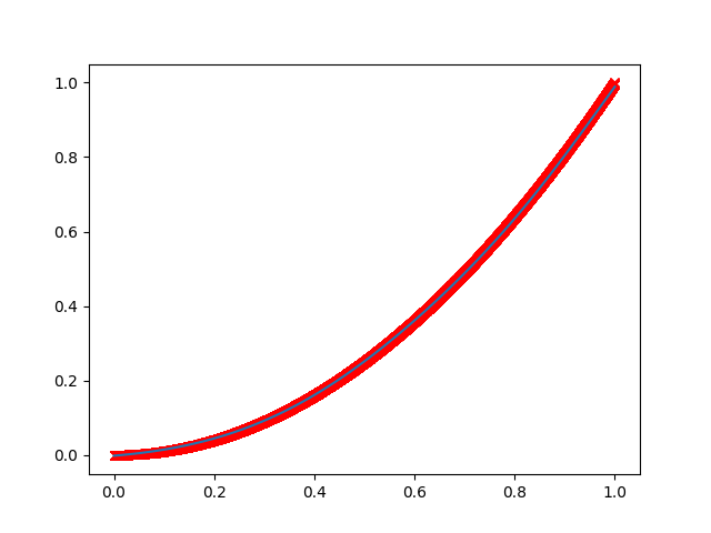
Ok, as a first case we create a net to fit some 1D data, that we put on a parabolic function.
The net will take a value of "x" as input and return its prediction for "y", which should be x squared.
Let's define a net made of 3 hidden layers, of 5, 10 and 5 nodes (neurons) each.
import numpy as np
from keras.models import Sequential
from keras.layers import Dense
from keras import optimizers
from keras import metrics
from keras import losses

import matplotlib.pyplot as plt

# Create dataset of 10000 points
X = np.random.rand(10000,1)
Y = X**2

# Create neural net model with Keras
model = Sequential()
model.add(Dense(5, input_dim=1, activation = 'tanh'))
model.add(Dense(10, activation='tanh'))
model.add(Dense(5, activation='tanh'))
model.add(Dense(1, activation='linear'))

# Compile model (set parameters)
model.compile(optimizers.Adam(lr=0.01), loss=losses.mean_squared_error, metrics=['mse'])

# Fit the Keras model on dataset (using random values for epochs and batch_size here!!!!)
history = model.fit(X, Y, epochs=40, batch_size=50)

# Test the net
X_test = np.linspace(0,1,100)
Y_test = model.predict(X_test, batch_size=1)

plt.plot(X,Y,'xr')       # plot training data
plt.plot(X_test, Y_test) # plot predictions
plt.show()
Note that the training process is stochastic in nature.
By running the script more times, you may get different results, even quite different!
One result may look like this (sorry for the crappy quality):
Saving and loading the model (exporting the weights)
As we all know, every layer of a neural net is described by a matrix of weights and an offset (the bias).
The training process creates such elements.
Keras offers a simple way to save the weights in a h5 file:
# Save model
model.save('saved_keras_model.h5')
If you are using Octave / Matlab you can load this model using "load()" and access the structure of the
created object, which contains the weights and biases for every layer.
If you prefer to work by hand, here's what you can do:
# Get weights

# One possibility is this:
weights = model.get_weights() # returs a numpy list of weights

# Otherwise, you can do:
counter = 0
for layer in model.layers:
    print('+++++++++++++ Layer %d +++++++++++++++\n\n', counter)
    weights = layer.get_weights() # list of numpy arrays
    print('W = ', weights[0])
    print('b = ', weights[1])
    counter += 1
    print('\n\n++++++++++++++++++++++++++++++++++++++++++++++++++++++++++\n\n')
Note that the weights matrix W and the offset b may be transposed with respect to your notation!
One input - two outputs
It is possible to train the same network to retrieve two outputs, for example the square of the input parameter x, and its sine function, sin(N*pi*x).
The only modification consists in the last layer, which will be composed of two output notes.
In the following script, the data is imported from a CSV file, that contains "x" as the first row, then "x**2" and sin(N*pi*x).
import numpy as np
from keras.models import Sequential
from keras.layers import Dense
from keras import optimizers
from keras import metrics
from keras import losses

import matplotlib.pyplot as plt

# Import dataset. X goes from 0 to 1.
dataset = np.loadtxt('testsin.csv', delimiter=',')
X = dataset[:,0]   # First column is the input
Y = dataset[:,1:3] # Second and third column are the outputs for training

# Create neural net model with Keras
model = Sequential()
model.add(Dense(5, input_dim=1, activation = 'tanh')) # One input
model.add(Dense(10, activation='tanh'))
model.add(Dense(5, activation='tanh'))
model.add(Dense(2, activation='linear')) # Two outputs

# Compile the Keras model
model.compile(optimizers.Adam(lr=0.01), loss=losses.mean_squared_error, metrics=['mse'])

# Fit the Keras model on dataset
history = model.fit(X, Y, epochs=40, batch_size=50)

X_test = np.linspace(0,1,100)
Y_test = model.predict(X_test, batch_size=1)

plt.subplot(2,1,1) # Print first output Y
plt.plot(X,Y[:,0],'xr')
plt.plot(X_test, Y_test[:,0])

plt.subplot(2,1,2) # Print second output Y
plt.plot(X,Y[:,1],'xr')
plt.plot(X_test, Y_test[:,1])

plt.show()
If you inspect very carefully the prediction, you may see that in the supposedly parabolic solution there is some oscillation that
reminds the second sinusoidal prediction.
In the end, the two predictions come from the same matrices, through an optimization process that keeps them quite mixed up.
This is not clearly evident, though.
Scaling the data
Neural nets are usually formulated such that the output of every neuron is a linear combination of the previous layer, but scaled to unity by a sigmoid function.
Therefore, the output of a net formulated in such way is bounded and cannot reach whatever value.
However, probably Keras autmatically does some rescaling, since it is able to retrieve values much larger than 1 and larger than the dimension of the last layer!
Still, it is always a good idea to rescale the data to a unitary range, as this helps the optimization quite a lot.
For example, if we would add "+200" to the output data of the previous network, we would get some very bad result, such as this one:
The scaling can be done in a simple way, as shown in the next figure.
Note that you should scale all variables!
So here is a way to do this scaling:
# Rescaling data
Xmin   = np.min(X[:])
Xmax   = np.max(X[:])

Ymin_0 = np.min(Y[:,0])
Ymax_0 = np.max(Y[:,0])

Ymin_1 = np.min(Y[:,1])
Ymax_1 = np.max(Y[:,1])

for ii in range(np.size(X)):
  X[ii]   = (X[ii]   - Xmin)/(Xmax - Xmin)
  Y[ii,0] = (Y[ii,0] - Ymin_0)/(Ymax_0 - Ymin_0)
  Y[ii,1] = (Y[ii,1] - Ymin_1)/(Ymax_1 - Ymin_1)


# Create neural net model with Keras
model = Sequential()

[.....] # COMPILE MODEL, TRAIN ETC ETC ETC....

# Now use the test to predict data
X_test = linspace(0,1,100)
Y_test = model.predict(X_test, batch_size=1)

# Re-scale the net output to the original range
for ii in range(np.size(X_test)):
  X_test[ii]   = Xmin   + X_test[ii]*(Xmax - Xmin)
  Y_test[ii,0] = Ymin_0 + Y_test[ii,0]*(Ymax_0 - Ymin_0)
  Y_test[ii,1] = Ymin_1 + Y_test[ii,1]*(Ymax_1 - Ymin_1)
And here is the result, properly working as expected.
Note that the average is around 200.
Fitting exponentials
Fitting functions that show an exponential behavior, or functions spanning many orders of magnitude is quite tricky and may
lead to a bad reproduction of some ranges of data.
A solution consists in
- Shifting the function such that the minimum value is 1;
- Computing the logarithm of the function.
The scaling is shown in the next picture
The logarithm of the function will be our new dataset, and we still have to rescale it to unit range at this point.
Then, we train the network upon it.
Fitting 2D data
Fitting 2D data, such as a function f(x,y) = x**2 + y**2 - 3*x*y is quite trivial.
You just have to provide 2 inputs to the first layer, here x and y, and one output result.
Here's the script:
import numpy as np
from keras.models import Sequential
from keras.layers import Dense
from keras import optimizers
from keras import metrics
from keras import losses

import matplotlib.pyplot as plt  # You may want this for plotting
from mpl_toolkits import mplot3d # You may want this for plotting

# Create dataset
Ntrain = 1000
X = np.random.rand(Ntrain)
Y = np.random.rand(Ntrain)
Z = X**2 + Y**2 - 3*X*Y

XY = np.zeros((Ntrain,2)) # initialize

# Rescaling data
Xmin   = np.min(X)
Xmax   = np.max(X)

Ymin = np.min(Y)
Ymax = np.max(Y)

Zmin = np.min(Z)
Zmax = np.max(Z)

for ii in range(np.size(X)):
  X[ii]   = (X[ii]   - Xmin)/(Xmax - Xmin)
  Y[ii]   = (Y[ii]   - Ymin)/(Ymax - Ymin)
  Z[ii]   = (Z[ii]   - Zmin)/(Zmax - Zmin)

  XY[ii,0]  = X[ii] # Create the 2D array
  XY[ii,1]  = Y[ii]

# Create neural net model with Keras
model = Sequential()
model.add(Dense(5, input_dim=2, activation = 'tanh'))
model.add(Dense(10, activation='tanh'))
model.add(Dense(5, activation='tanh'))
model.add(Dense(1, activation='linear'))

# Compile the Keras model
model.compile(optimizers.Adam(lr=0.01), loss=losses.mean_squared_error, metrics=['mse'])

# Fit the Keras model on dataset
history = model.fit(XY, Z, epochs=40, batch_size=50)
You can see that in the script we are training on 1000 points only.
This still works very well, as you can see in the next image.
Sorry for the poor quality... it works, the mismatch is just visual :-)
More tough 2D data: exponentials
So, as previously described, if you want to fit exponential functions, you should do a logarithmic scaling of the data
before feeding it to the training algorithm.
The log scaling greatly reduces the span of the function, limiting its variations in terms of orders of magnitude.
Moreover, if we are trying to fit a purely exponential function, such as "exp(x**2 + y**2)", then the log scaling makes this
function linear!
This means that the neural net will be trained on a plane.
This is a remarkably simple task, such that we really need a minimal net to get this result done, and a minimal set of data!
Check out the script, here
This script will also compute the maximum and minimum relative errors (percentage) to give you an idea of how good your
neural network predictions are.
Also, it plots the relative error, and you can see that it really gets small!
Lesson learned here:
all the pre-digestion that you can do on your data will be of great use for the training.
The simplest the data, the better the fit.
If you have some physical data and you have some physical intuition for what is going on there, use this intuition to
rescale the data, as to make everything as linear as possible.
Then scale it back.
Back to Homepage