Numerical integration in C++ with Boost odeint

• Boost v1.60 library page on integration
• Odeint examples
• Odeint tutorials

0 - Integration functions

1. integrate_const
2. integrate_n_steps
3. integrate_times
4. integrate_adaptive
5. integrate

• stepper is the mathematical scheme you wish to use (such as Runge-Kutta or Euler). It defines how the integration is to be made: constand steps, adaptive, stiff systems etc
• system is a function implementing the mathematical system (or the scalar equation) you want to solve. This function takes as an input the current state and time and creates the time derivative dxdt
• x0 is the initial condition
• t0 and t1 are initial and final times for integration
• dt is a timestep, but its signifiance depends on the type of stepper
• observer this is a function that is called every N timesteps, that you can use to print intermediate solutions. It's optional. Without it the integrator will just integrate from t0 to t1 and then return with no useful output

1 - Simplest ODE problem

 #include <iostream>
 #include <boost/numeric/odeint.hpp>       // odeint function definitions 
 
 using namespace std;
 using namespace boost::numeric::odeint;
 
 // Defining a shorthand for the type of the mathematical state
 typedef std::vector< double > state_type;
 
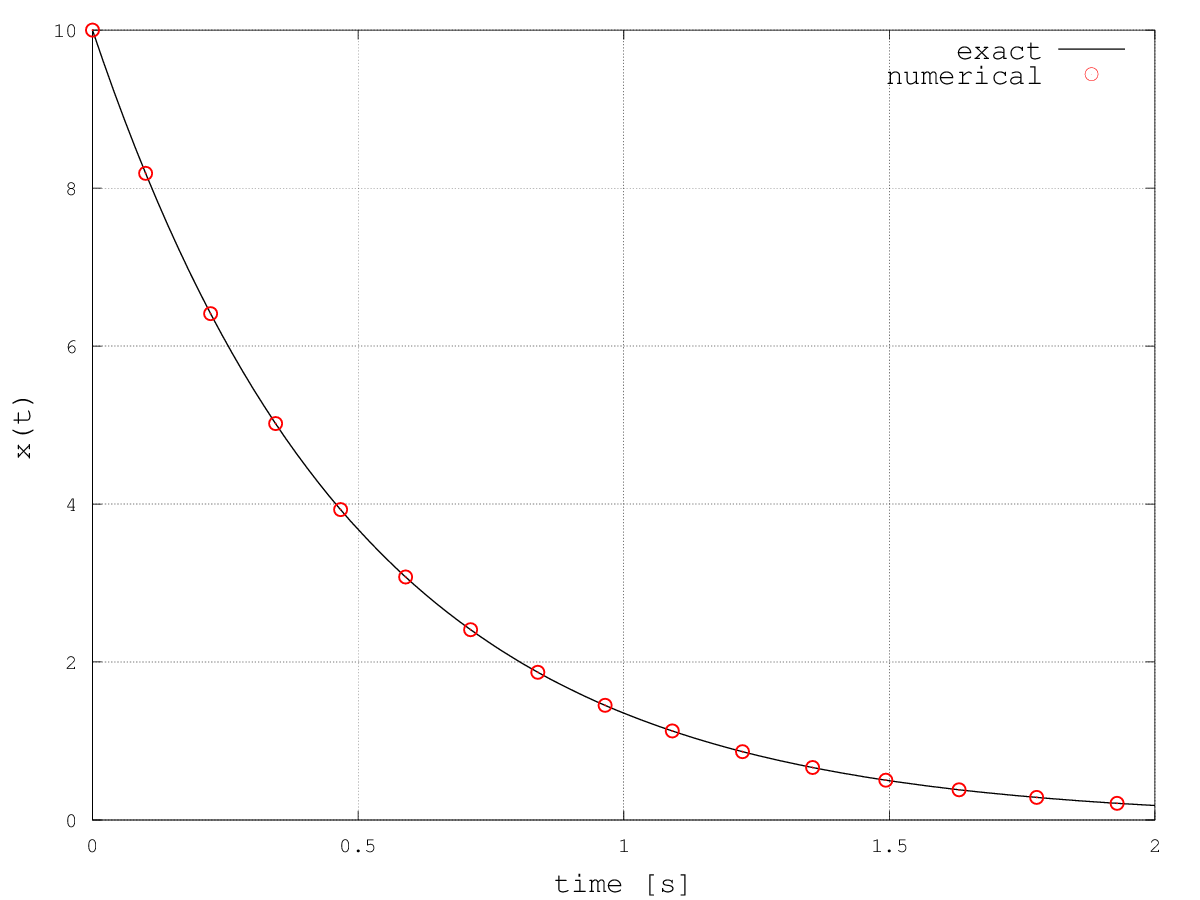
 // System to be solved: dx/dt = -2 x
 void my_system( const state_type &x , state_type &dxdt , const double t )
 {    dxdt[0] = -2*x[0];   }
 
 // Observer, prints time and state when called (during integration)
 void my_observer( const state_type &x, const double t )
 {    std::cout  << t << "   " << x[0] << std::endl;   }
 
 // ------  Main
 int main()
 {
     state_type x0(1); // Initial condition, vector of 1 element (scalar problem) 
     x0[0] = 10.0;
 
     // Integration parameters
     double t0 = 0.0;
     double t1 = 10.0;
     double dt = 0.1;
 
     // Run integrator
     integrate( my_system, x0, t0, t1, dt, my_observer );
 }

1. First of all, as you can see the integrate function does not require a stepper. In fact, integrate is the simplest integration function, used just to perform some integration on the fly. You usually want to use the others (see below).
2. Secondly, you should note that the solution of the mathematical problem, x (aka the "state" of the system) have a type that we called state_type. One can choose various different types, here I've opted for a simple std vector of doubles, whereas we could have used ublas types for example.
3. The my_system function takes as an input the current state and fills the second argument, dxdt that is the left hand side of the ODE problem.
4. The observer just prints the intermediate result. We could have used it to write the results on a file.
5. The observer is invoked roughly every "dt".

2 - Integration functions: overview

• integrate_const calls the observer at equidistant times separated by dt. The syntax is:
  integrate_const( stepper , system , x0 , t0 , t1 , dt , observer )
• integrate_n_steps is like the previous one but does not ask for the end time, instead it asks for the number of timesteps to integrate. Syntax:
  integrate_n_steps( stepper , system , x0 , t0 , dt , n , observer )
• integrate_times performs integration at given timesteps. Syntax:
  integrate_times( stepper , system , x0 , times_start , times_end , dt , observer ) integrate_times( stepper , system , x0 , time_range , dt , observer )
• integrate_adaptive is used if you want to call the observer at each timestep. Syntax:
  integrate_adaptive( stepper , system , x0 , t0 , t1 , dt , observer )
• integrate this is the "convenience integrate function", simple and quick to set without need to specify a stepper. Syntax:
  integrate( system , x0 , t0 , t1 , dt , observer )

3 - Integration with steppers

 integrate_const( runge_kutta4<state_type>(), my_system, x0, t0, t1, dt, my_observer );

 typedef runge_kutta4<state_type> rk4;
 integrate_const( rk4(), my_system, x0, t0, t1, dt, my_observer );

 // ------  Main
 int main()
 {
   state_type x(1); // the state, vector of 1 element (scalar problem)
   x[0] = 10.0;
   
   // Integration parameters
   double t = 0.0;
   double dt = 0.1;
   size_t nSteps = 1000;
   
   // Create stepper
   runge_kutta4<state_type> rk4;
   
   // Perform integration step by step
   for(int ii = 0; ii < nSteps; ++ii)
   {
     // adjourn current time
     t += dt;
   
     // now perform only one integration step. Solution x is overwritten
     rk4.do_step(my_system, x, t, dt);
   
     // ... and output results
     cout << t << "   " << x[0] << endl;
   }
 }

• basic stepper
• error stepper
• controlled stepper
• dense output stepper

#include <iostream>

#include <boost/numeric/odeint.hpp> // odeint function definitions

using namespace std;
using namespace boost::numeric::odeint;

// Defining a shorthand for the type of the mathematical state
typedef std::vector< double > state_type;

// System to be solved: dx/dt = -2 x
void my_system( const state_type &x , state_type &dxdt , const double t )
{
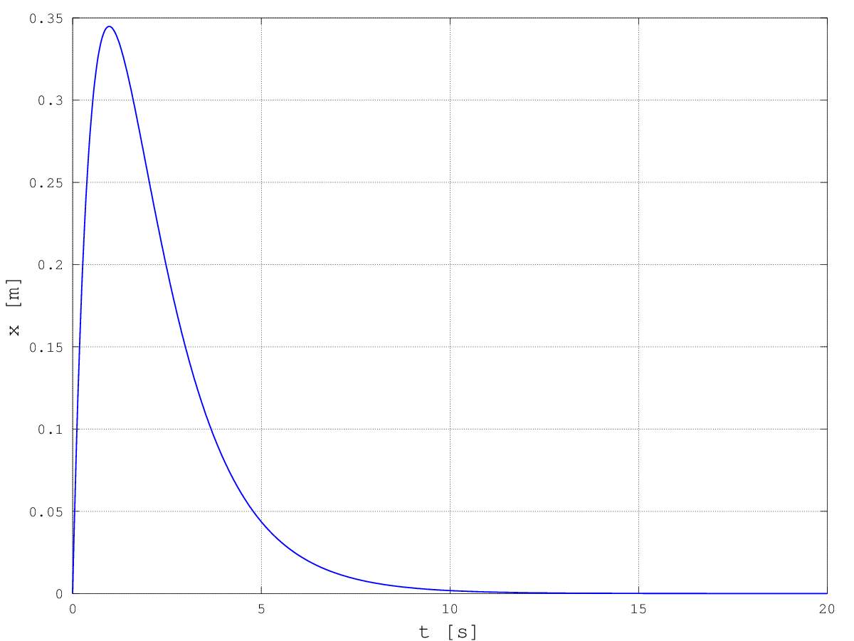
    dxdt[0] =  0*x[0]  +   1*x[1];
    dxdt[1] = -1*x[0]  - 2.2*x[1];
}

// Observer, prints time and state when called (during integration)
void my_observer( const state_type &x, const double t )
{
    std::cout  << t << "   " << x[0] << "   " << x[1] << std::endl;
}

// ------  Main
int main()
{
    state_type x0(2); // Initial condition, vector of 2 elements (position and velocity)
    x0[0] = 0.0;
    x0[1] = 1.0;

    // Integration parameters
    double t0 = 0.0;
    double t1 = 20.0;
    double dt = 1.0;

    // ----  Steppers definition  ----
    // Basic stepper:
    // follows given timestep size "dt"
    typedef runge_kutta4<state_type> rk4;

    // Error stepper, used to create the controlled stepper
    typedef runge_kutta_cash_karp54< state_type > rkck54;

    // Controlled stepper: 
    // it's built on an error stepper and allows us to have the output at each 
    // internally defined (refined) timestep, via integrate_adaptive call 
    typedef controlled_runge_kutta< rkck54 > ctrl_rkck54;

    // ----  Run integrations with the different steppers  ----

    // Run integrator with rk4 stepper
    std::cout << "==========  rk4 - basic stepper  ====================" << std::endl;
    integrate_adaptive( rk4(), my_system, x0, t0, t1, dt, my_observer );

    // Run integrator with controlled stepper
    std::cout << "==========  ctrl_rkck54 - Controlled Stepper  =======" << std::endl;
    x0[0] = 0.0; // Reset initial conditions
    x0[1] = 1.0;
    integrate_adaptive( ctrl_rkck54(), my_system, x0 , t0 , t1 , dt, my_observer );
}

• I've choosed the integrate_adaptive integration function, that calls the solution also at intermediate timesteps, so that we can see how the controlled stepper works.
• When a controlled stepper is passed to integrate_adaptive, the timestep dt is just an initial guess timestep. This timestep as well as all the others can be refined with error criteria, in fact you can see from the plot at right that despite the timestep was initially set to dt = 1.0, at the end of the controlled stepper integration the actual step is bigger!

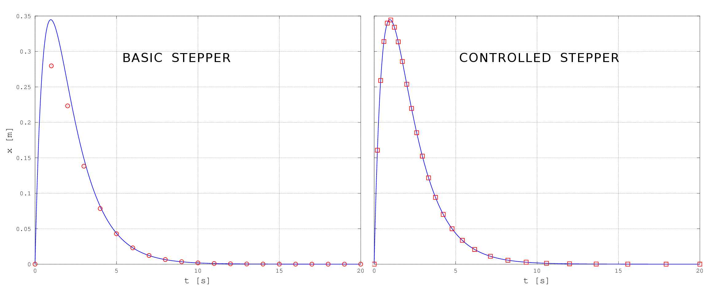
==========  rk4 - basic stepper  ====================
0   0   1
1   0.279667   0.0914
2   0.223193   -0.0698595
3   0.138185   -0.0688047
4   0.0784087   -0.0449346
5   0.0428421   -0.0260353
6   0.0229939   -0.0143611
7   0.0122327   -0.00774322
8   0.00647889   -0.0041288
9   0.00342373   -0.0021893
10   0.00180716   -0.00115761
11   0.000953317   -0.000611208
12   0.000502743   -0.000322475
13   0.000265086   -0.000170075
14   0.000139763   -8.96806e-05
15   7.36854e-05   -4.72839e-05
16   3.88473e-05   -2.49291e-05
17   2.04802e-05   -1.31428e-05
18   1.07971e-05   -6.92889e-06
19   5.69216e-06   -3.65289e-06
20   3.00087e-06   -1.92578e-06
==========  ctrl_rkck54 - Controlled Stepper  =======
0   0   1
0.2   0.160729   0.62909
0.4   0.25906   0.369921
0.6   0.314033   0.191075
0.809566   0.339954   0.065062
1.01913   0.344383   -0.0166857
1.2428   0.33413   -0.0702323
1.47763   0.31359   -0.101238
1.73025   0.285836   -0.11597
2.00191   0.253734   -0.118652
2.29508   0.219629   -0.112967
2.6131   0.185377   -0.101919
2.96069   0.152372   -0.087867
3.34299   0.121725   -0.0726501
3.76712   0.0941826   -0.0576185
4.24293   0.0702024   -0.0437071
4.78465   0.049993   -0.0315045
5.41432   0.0335592   -0.0213196
6.17034   0.0207314   -0.0132375
7.13966   0.0111524   -0.00714214
8.2138   0.0056026   -0.0035926
9.33462   0.00272999   -0.00175145
10.5825   0.0012258   -0.00078657
11.998   0.00049426   -0.000317177
13.6366   0.000172728   -0.000110845
15.5745   4.98493e-05   -3.199e-05
17.9281   1.10743e-05   -7.10652e-06
20   2.9352e-06   -1.8835e-06

// Define the error stepper
typedef runge_kutta_cash_karp54< state_type > error_stepper_rkck54;

// Error bounds
double err_abs = 1.0e-10;
double err_rel = 1.0e-6;

// Fire! 
integrate_adaptive( make_controlled( err_abs , err_rel , error_stepper_rkck54() ) , 
                    my_system , x0 , t0 , t1 , dt , my_observer );

4 - Stiff problems and Jacobian

Stiff problems are characterized by very different timescales. Think for example at a chemically reacting mixture: chemical rates may be very different among each others (by orders of magnitude!) That characteristic makes common integrators inappropriate and one needs apposite solvers.
Consider for example the following system:

This is basically a system where the derivative of the first component x1 is likely way bigger than the one for the second component x2. A quick check with matlab shows that a Runge-Kutta 45 adaptive method (ode45) takes 70000 steps to solve it into a certain interval, whereas a stiff solver (ode15) takes only 100 timesteps!
The more the system stiffness, the more the disparity: what if we increase the stiffness, then? Let's put the coefficients of the first equation to 30000 and 20000, the required timesteps for the nonstiff solver increase to 700000, while the stiff solver takes still 100 timesteps!!! Of course, nobody knows what kind of black magic they put into Matlab functions, but I think you are now convinced of the importance of stiff solvers.

Odeint implements some stiff solvers, such as the rosenbrock4, but they additionaly require to provide the system Jacobian, that is the matrix of the partial derivatives. Also, note that the stiff integrator of Odeint *requires* that the system state is of ublas::vector type and the jacobian *must* be a ublas::matrix!

Here's a program that solves the problem defined above. Note that:

• I'm using a slightly different syntax for the system this time, not defining it as a function, but using functors: the system is defined as a structure and the operator "()" is overloaded so that when it is called with parenthesis it behaves like a function.
• The Jacobian too is defined as a struct, in the very same way as my_system
• I've used integrate_const, that differs from the previously used integrate_adaptive only in that we obtain the output precisely at each "dt"
• In the observer I use the std function setw(), that gives a slightly more cute output.

 #include <iostream>
 
 #include <boost/numeric/odeint.hpp> // odeint function definitions
 
 using namespace std;
 using namespace boost::numeric::odeint;
 
 // Defining shorthands for boost types vector and matrix.
 // vector is used for the system state "x" and matrix for the jacobian "J"
 typedef boost::numeric::ublas::vector< double > vector_type;
 typedef boost::numeric::ublas::matrix< double > matrix_type;
 
 // System to be solved.
 // This is a functor: "operator()" overloads the operator "()" making the
 // struct behave like a function
 struct my_system
 {
   void operator()( const vector_type &x, vector_type &dxdt, const double t)
   {
     dxdt[0] = -3000*x[0] -2000*x[1];
     dxdt[1] =    -2*x[0]    -3*x[1];
   }
 };
 
 // Jacobian of the system.
 // Functor! See struct "my_system"
 struct jacobian
 {
   void operator()( const vector_type &x, matrix_type &J, double t, vector_type &dfdt )
   {
     J(0,0) = -3000;
     J(0,1) = -2000;
     J(1,0) = -2;
     J(1,1) = -3;
   }
 };
 
 // Observer, prints time and state when called (during integration)
 void my_observer( const vector_type &x, const double t )
 {
   std::cout << t << setw(15) << x[0] << setw(15) << x[1] << std::endl;
 }
 
 // ------  Main
 int main()
 {
   vector_type x0(2); // Initial condition, vector of 2 elements (position and velocity)
   x0[0] = 0.0;
   x0[1] = 1.0;
 
   // Integration parameters
   double t0 = 0.0;
   double t1 = 20.0;
   double dt = 1.0;
 
   // ----  Run integrations with the different steppers  ----
 
   // Stiff integration
   integrate_const(make_dense_output< rosenbrock4< double > >(1.0e-6, 1.0e-6),
                   make_pair(my_system(), jacobian()),
                   x0, t0, t1, dt, my_observer);
 }

Back to HOMEPAGE