Compressible flows and the CFL condition
Back to HOMEPAGE
References:
Randall Leveque, Numerical Methods for conservation laws
Compressible Fluid Dynamics problems are mathematically different
then incompressible ones, in that they show a limited speed of propagation of perturbations.
Perturbations propagate in the domain as waves and since their velocity is finite there might
be some portion of the domain that is unaware of what is going on somewhere else.
This is a well known behaviour of supersonic flows.
Another way to express this idea is saying that the problem is "local".
By contrast, incompressible fluid dynamic equations show infinite velocity of propagation
of perturbations and the problem becomes "non-local":
if you try to perturbate somewhere your incompressible flow, every point in the domain will
istantaneously feel the perturbation.
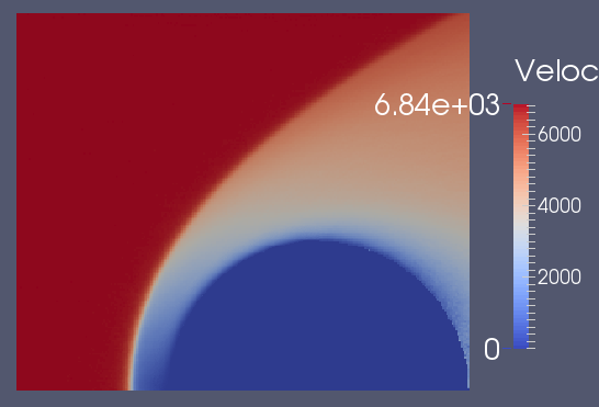
In the figure, a supersonic (actually, hypersonic!) flow around a cylinder. The upstream flow before
the shock wave doesn't know anything about the incoming ball.
Let's neglect for a moment the viscosity and try to numerically simulate the (simpler) Euler's
gas dynamics equations, that are a set of hyperbolic equations.
Another very famous hyperbolic equation is the wave equation, another one being the Burgers' equation
and the traffic equation.
All those equations have something in common with the Euler' equations: finite velocity of propagation of
informations.
Solving hyperbolic equations requires a totally different approach with respect to elliptic
and parabolic PDEs, the reason being that hyperbolic problems can show jumps in the solutions.
The solution of linear scalar hyperbolic equations fetched with discontinuous
initial conditions is the propagation of the initial jump, whereas nonlinear equations (such as the
Burgers' equation or the Euler's equations) may develop "jumps" also if fetched with smooth initial conditions.
In case of the Euler's equations, those jumps are usually called "shock waves".
The speed of jumps (and shock waves) may be different from the speed at which perturbations propagate and
can be found on the grounds of conservation criteria.
Since hyperbolic problems may naturally give rise to discontinuous solutions, one should not look at them
as "just a PDE problem", but should remember where they were obtained from (conservation principles!) and
refrain from committing the usual step "let's transform this surface integral using the divergence theorem!"
Do you remember when to obtain the Navier Stokes momentum equation you wrote down that the flux of momentum
across the boundary of a domain is equal to the volume integral of the divergence?
This step requires the solution to be differentiable, which is not the case as we said!
The solution of hyperbolic problems is better searched in the world of the so-called weak solutions,
that satisfy integral problems (not PDEs).
It might not be so bad.. After all, integral problems are closer to physics since they are the direct mathematical
transposition of conservation principles, aren't they?
So, how do we numerically simulate those happily-jumping solutions?
By, as said, going back to the integral conservation problem!
Let's think of a 1D problem to fix the ideas.
We could split the x axis into some pieces (that we call cells), approximate the solution on those (small) pieces
as constant and solve the integral conservation equations among them.
Doing that is not hard and means computing the fluxes exiting one cell and entering another.
This is basically the idea of the Godunov method, that solves the Euler's equations by approximating it
with a series of Riemann problems, and could be mapped in 3 dimensions giving rise to finite volume schemes.
Note that the formulation of the numerical fluxes can be done in such a way that the resulting scheme has the same
exterior appearence of a finite difference upwind method for example!
In those methods there is a condition called "CFL condition" to be respected in order for the method to
converge (it is a necessary, non sufficient condition).
The CFL condition states that the space travelled by characteristic lines in a timestep dt must be smaller
then the length h of a cell.
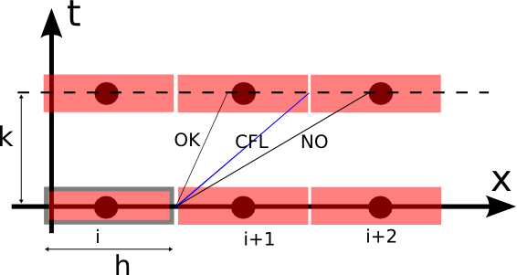
In the above picture, the x axis is divided in red cells (in the center of which I depicted a "grid point").
The length of each cell is h, that is also the distance between two "grid points".
At each timestep fluxes leave one cell and enter the next one.
The characteristic velocity is the angle created by the inclined lines starting at the interface of two cells.
Now note the significance of the CFL condition: if the timestep is too big with respect to the characteristic
velocity, then in one timestep the flux have not only entered one cell (the i+1) but have also entered
the next-next one (the i+2).
This case is not modelled by our solver, that attributes an outgoing flux to the adjacent cell only and
thus not respecting the CFL conditions means that we are not properly simulating the physics of the problem!
Back to HOMEPAGE